Another good day, and some more good data

I'll be brief - Today we filled in a bit of the area that we had missed on the previous days, in addition to getting some detailed measurements directly over the bubbling CO2 springs.  Below is the updated track map, followed by the measured CO2 concentration map

You can see 5 hot spots, which are essentially the springs area covered in one of the traverses.  The CO2 and d13C time series profiles for the traverse that covered those areas is shown below. Clearly, we are now getting the kind of data that we have been looking for.

 I haven't gone too far into the interpretation, but the CO2 concentration increase seems to correspond with an increase in the isotopic signature of the gas.  The increase is fairly modest for the given concentration increases, and past studies have found that the d13C of exsolving gas has a value of -6, just positive of atmospheric.  So in a sense, this is what we would expect. We will have to do a lot more processing and analysis back home to put some quantitative analysis to this.

Tomorrow is likely our final day of surveying and the goal is to do a high resolution measurements over the springs area and pin down exactly over how much area the leaking CO2 can be detected.

No more bad weather

Some pictures

William leading the instrument mule on our first good day.

Our trucks, coming through the mud.

Data

The first ever Abstract to a blog post:
We have taken CO2 concentration and 13C isotopic signature measurements across an area of approximately 2.5 km^2 with about 22 km of traverses.  CO2 signatures were as expected (360 ppm, d13C = -8 for the majority of the survey) We have 1 clear signal from a "hotspot" CO2 source, while other would-be observations were fouled by pulling water into the sampling tube.  Pulling water into the sampling tube presents a number of problems including fouling the measurements and potentially damaging the equipment and a new design for the sampling tube has been implemented for the next days.  In addition, the survey goal has been refined to produce a high resolution dataset for the area of known seepage activity.

We got in a couple of hours of surveying on saturday and a full day on yesterday and finally have some good data to analyze.  It's a really rainy day today so as Lin finds his way home, we are sitting in the Green River Coffee Company with everyone else in town, working on the data.

The green line in the map above shows our saturday path, and the burgundy line shows yesterday's. Despite the near perfect weather, saturday's survey was cut short when the mule carrying the instrument briefly bolted as we traversed the area of CO2 seepage. Nothing was damaged, but a tube that is used to keep a vacuum in the instrument snapped at its fitting, and it was a repair that could only be made back at the hotel.  In addition, we got a truck stuck in deep mud yet again which would have prevented us from receiving a relief battery if the tube issue hadn't come up anyway.  Logistical problems have been limiting our progress and Lin, Taku, and I had a big discussion on saturday night to strategize how to avoid these issues in the following days. More on that later.

Yesterday, however, was a different story. We managed to paint 2.5 km^2 with 16 km of traverses in about 5 hours of surveying.  The terrain is both soft ground and high relief for walking (see the elevation profile below) and this seemed to be about what we could do without driving the animals too hard.  For the final 2.5 miles, we got off and walked with the mules to give them a little boost at the end.

The above graph plots the CO2 concentration in ppm for the traverses (latitude and longitude). Note that the map is slightly different as it was taken with the coordinates of the path that the instrument actually took while it was logging data, whereas the first image shows the coordinates taken with the GPS I was holding.  There are a couple interesting observations.  The dark red area consists of a series of measurements of CO2 concentration above 1400 ppm (see below) which apparently started as the machine was walked over the large bubbling spring.  The red track stops when the mule bolted and measurements were effectively halted for the day, unfortunately.

The below graph shows the CO2 concentration profile and d13C profile as we moved over that location.     The initial drop in d13C signature is a typical startup profile for the machine, which makes the initial 3-4 minutes of d13C data throwaway.  It is interesting that after that, while the 12C concentration is very stable, the d13C signature is highly variable until 18:56 when we hit a hotspot.  I haven't found any particular source for this fluctuation and am looking into it further.  After that, the d13C signature stabilized at around -9 while the CO2 concentration seems to be slowly drifting downward.  My interpretation of this is that we hit the hot-spot, but because the tube was dragging on the ground, it pulled in some liquid water.  Thus, the initial spike in CO2 concentration was sustained because the plug of liquid water provided a reservoir of CO2 as it vaporized into the measurement chamber.

There is another interesting area of high CO2 concentration on the northern most traverse that crosses the -110.11 line.  The CO2/d13C profile for that is shown below.

That long light blue to green traverse is the result, again, of pulling water into sampling tube.  What is particularly frustrating about this one is that this took place right before we went over the area of the springs and didn't catch that the data was bad until too late. We will, however, be going back (see a subsequent post on plans moving forward) to the springs and raising the sampling tube on the leg of the mule proved for the rest of the day to have eliminated the problem of pulling water into the tube.

Before anyone gets too excited, the single red spot of high CO2 concentration is a location where I breathed into the tube to check that it was indeed sampling correctly after I had put it up a bit higher on the mule's leg.

In summary, we have taken a lot of good measurements covering a wide area around the location of known CO2 seepage.  We need to take another round of very detailed and non-fouled measurements over the known CO2 seepage itself to obtain a high-quality positive leakage signal.

Finally, the elevation profile below:

Rainy day, a scare, and some redemption

Today was tough. Contrary to popular opinion, it does rain in Green River, and while I wouldn't say the forecast got the timing exactly right, it is clear that the general warning is something to take note of. 

The rain was not too hard, and didn't prevent us from surveying, we did a 3-hour ride taking measurements today.   It did, however, turn the dirt access roads to a mud with the texture of warm butter.  This, you can imagine is very difficult to drive on, and we spent quite a bit of time dealing with getting stuck in various places, and did not get to the start of the targeted area of CO2 seepage.  If it continues to rain, it will be somewhat of an issue as it essentially cuts off our access to some areas deeper into the Salt Wash in addition to generally slowing us down.  We have a strategy moving forward to survey areas that are easily accessible in the rain while it is raining and to bolt for the difficult to access areas on the days where we have dry weather.

The other major problem that came from the rain was the impact of sucking water into the sampling tube on the measurements.  This gave us a pretty big scare today as our measurements essentially stopped making any sense, and the problem persisted even running the instrument in the hotel room.  Chris of Picarro, who I have now Canonized as St. Rella, helped me through a process which essentially required opening up the instrument, taking out a piece that had collected the water, and shaking it dry.  It was fairly simple in practice and it entirely fixed the problem.  We can avoid getting water in the system in the first place by lifting the inlet tube up when we walk through the small streams that have now popped up in the area.

Finally, we did have some redemption, as we now think we have solved the puzzle of the rapidly fluctuating CO2.  We ran some tests in the hotel room where we turned the instrument on, held it in the position that it sits in the saddle-bag, and shook it with a rhythm approximating the gait of a mule.  The inlet tube was sticking out the window of the hotel room.  It turned out that if we were facing the instrument while we were shaking it, there were large fluctuations in the CO2 concentration.  If we held the instrument behind our back while we were shaking it, there were no fluctuations.  It just means that the fitting between the sampling tube and the instrument is not tight, and leaks particularly when it is shaken.  Because where this connection is made on the instrument is near to the mule's breathing, we see the rapid fluctuations in CO2 accordingly.  The fluctuations disappear when the mule is standing still .  If this is truly the last piece to the puzzle, it is an easy fix, and we will have some good news tomorrow.

Lin has arrived, so we have a strong team going into the weekend. Wish us luck! 

Data from the practice run

The below map shows where we rode today with the mule along with an elevation profile of that ride. Today's track is in burgundy.  The green track shows yesterday's ride and the bright red box shows where the obvious CO2 seepage is.  Essentially we parked where the Ruby Ranch Road intersects the Salt Wash, set up our gear, and went on a practice ride from there.

The practice ride was 4.22 miles. We covered that in about 2 hours, which makes for a typical walking pace of just over 2 mph.  This is somewhat slow for the ground we would like to cover, but during this ride we stopped several times to check out the data, try out various configurations with the inlet tubing, and investigate the source of somewhat unexpected rapid fluctuations in the absolute CO2 concentration (see below).  We also underwent a lot of elevation gain and loss, and this is something that we will also not be doing during surveying days. William led today, and I essentially asked that he take us through distinctly different types of terrain, including bushes and some steep stuff, to test if it made any impact on the measurements.  Survey days will be broken up into blocks in which we cover a relatively flat area in a bench or valley, move up or down to a neighboring bench or valley, survey, and move on again.

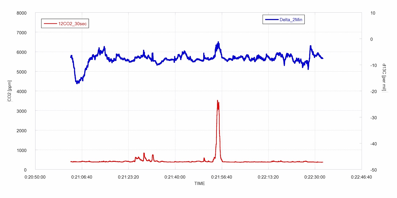
Here is a look at the data that we collected on this ride. The graph shows the CO2 concentrations [ppm] in red and with the y-axis on the left.  Corresponding Delta 13-C signatures [per mil] are shown in blue with the y-axis on the right.  

The CO2 concentrations fluctuate from 370 ppm to about 480 ppm, with a handful of isolated points breaching that.  This is a much wider range than we were expecting.  For some comparison, in Montana, surveying areas in an alfalfa field away from areas of CO2 leakage, CO2 concentrations ranged from 373-376 ppm.  The isotopic signature is noisy because of the rate of fluctuation of the CO2 concentration, but on average has a value of exactly what we would expect from atmospheric CO2: -8. 

We have two other piece to this puzzle: (1) when the mule was standing still, the CO2 concentrations are relatively flat; Essentially every place in the below graph that has a flat concentration is a time when the mule was standing still. (2) While nearly all the data was taken with the tube inlet attached to the mule's ankle, the last 10 minutes of data are taken with the sample inlet sticking up out of the machine above the mule.  

There are several potential causes for this data: (1) The fluctuation is natural from background sources, either large volumes of CO2 are exhausting from soil gas (it was a cloudy day), or from prevalent CO2 leakage in the area (2)  There is some noise introduced into the instrumentation as a result of it shaking while the animal is moving (3) Animals breathing are polluting the signal.

 Chris of Picarro explained that vibrations will introduce random error in the concentration measurement through perturbations to the pressure of the measurement chamber in the instrument. The error introduced follows the law: deltaC/C = 1/6*deltaP/P.  Below is a graph of the CO2 concentration and the pressure in the chamber (in torr) on the same time axis:

It is clear that there are pressure perturbations due to the movement of the animal, but they are quite small.  The standard deviation of the pressure in the chamber around the targeted 140 torr is 0.4 torr during the times when the mule is moving.  For comparison, the standard deviation around the target pressure during our survey in Montana was about 0.2 torr.  This would correspond to a few ppm at most error in the concentration measurement, not the 20-100 ppm that is fairly frequent the above data.  In addition, the concentration fluctuation is always in the positive direction, while the pressure perturbations are evenly distributed around the mean and would result in both positive and negative error in the concentration measurement.

That the concentrations are fairly uniform when we are standing still seems to rule out natural background fluxes, and so right now I think that animals breathing is the strongest candidate.  We can test this tomorrow, checking to see what the isotopic signatures is of the animal breath, and also attempting to snorkel the sampling tube well away from the animals.  At this point, suggestions and feedback are more than welcome.

Tomorrow's survey will focus on the areas of obvious CO2 seepage (the boxed red area in the above image), and so we will also observe what a leakage signal looks like in these measurements.

Dress rehearsal

Today we put the entire setup together, got it on the mule, and did a 2.5 hour ride taking measurements.  It was successful, although the data was somewhat different than expected. In this post, I will describe the setup. In a subsequent post, I will have a discussion about our initial data and also some modifications we have made in response to today's work.

First things first. Here is a picture of William with the fully loaded mule.  I had a moment of surprise when I saw it thinking that it looked awfully like the schematic I had drawn back at Stanford.

The instrument is packed vertically (nose down) into a hard-shelled aluminum saddle pack. We have foam packing on all sides of the instrument, in addition to the rubber shock absorbers between the instrument itself and it's metal confining frame.  The back end is sticking out which ensures that no cables or tubing are being stressed and that the computer can have proper ventilation.  We have an easy-to-deploy tarp tucked into one side and can simply pull it over the instrument if it looks like any kind of precipitation is imminent. We also may use it just to guard against dust as well.

The tube runs along the back of the mule, held in mostly by leather straps on the tack (saddle and bag rig) and is strapped in one place on the bottom of the leg.  This configuration withstood several miles of walking through varied terrain, including heavy bush (see below).  In addition, the mule was not bothered by the tubing.

We covered varied terrain, which included bushes, sandy dry river beds, and fairly steep slopes.  The instrument logged data throughout the entire run until the battery ran out of juice unexpectedly early.  More on that in a subsequent post.

Update on the weather

At this morning's kickoff meeting, John, Sena, and William unanimously agreed that the weather would not be an issue.  They mentioned that thunderstorms moving through the area may hit, but would be brief.  The survey may be halted for rain and avoidance of lightning, but it should only put us back the 30 minutes or so it takes for the storm to move through. So, we are bringing the rain gear with some anticipation that we may have to wait out some brief weather.

The Natural Superiority of Mules

Today was our first day out with the mules and it went very well.  We are clearly in good hands with John and Sena Hauer of Backcountry Mules, who literally wrote the book on riding mules. They have also hired William Hatfield of Green River to work with us for each day of the survey providing local knowledge and generally managing the mules; getting them to our starting point in the morning, and cleaning and feeding them in the evenings.

The access road to the field site is the Ruby Ranch Road, 13 miles East of Green River.  The Salt Wash itself begins about 9 miles down that road.  We drove into the Salt Wash to see how far into the survey area we could get before having to get out and ride.  We were able to get far enough in so that we can essentially drive to our starting point for each day of surveying.  This also means that we will generally be close to our vehicle where we can store extra food, water, and other supplies.  We tried out various configurations of the Picarro instrument in saddle bags to make sure it would fit, and took a long surveying ride to cover the ground that we are hoping to survey in more detail over the next 6 days.

This dotted line below shows a track of the ground that we covered today; We essentially covered the area of known CO2 leakage, which is bordered in red. This will also be the area we go to on our first full survey day on friday.

Here are some pictures of the CO2 seeps in that area.

Field hotel room

This is a picture of the equipment working and the Yankees not working.

Weather forecast

The weather forecast isn't ideal.  I'll know more about our options after this morning's meeting.

Green River

We have finally settled in to Green River after 888 miles of driving that has been alternately spectacular and mind-numbingly monotonous.  Green River is quaint in a good way, but the many shuttered restaurants and hotels suggest that it has seen better times.  The last two restaurants standing (Ray's Tavern and Tamarisk) are enthusiastically recommended by everyone in response to nearly any question ("Hardware store? Nope, but, Ray's Tavern has great burgers!").   

I also stopped by the history museum on a complete whim to check if they had any useful maps or books.  It seems like everyone here asks why you are here and after mentioning to a woman overseeing the small museum and shop that we were here on research, she answered "Oh, I know who you are. You're the guy from Stanford going to look at the CO2 near Crystal Geyser?"  After a few seconds of me just staring at her in complete disbelief, she explained that she was the mother of one of the mule handlers that is coming to help us tomorrow.  Leaving the museum she mentioned that if he was late, we should just give her a holler and she could get him up and moving.  Thanks Mom!

We have settled in to the lovely Robbers Roost which offers clean rooms, warm showers, high-speed internet, HBO, and all for $34 a night to boot. We are meeting John Hauer at Tamarisk tomorrow morning for breakfast, so I guess it will be Ray's Tavern this evening!

And good news from Stanford

Lin will be joining us over the weekend.

Good news from Backcountry mules

I spoke to John Hauer of Back Country Mules this evening to finalize logistics for wednesday. It looks like they have hired someone to work with us during the days that John and Sena are not there, so we'll never be alone with the mules. In addition, we won't need to tow the trailer any more which means (1) we don't need to tow mules and (2) we don't need to rent an extra truck.

Road Trip

Here is how we are making our way across the West. From Stanford to Ely in one big push on the first day (530 miles or so).  Ely to Green River (another 250) the following.  As John Hauer of Back Country Mules mentioned this evening: We're finding out just how much space is between California and Utah.

Equipment

The following schematic is our going conception of how the instrument and auxilary equipment will be held in the saddle bags.

A few key changes have been made to the equipment setup since Montana.  Here, and below, you'll see that we have added a structural framework around the Picarro Instrument to protect it. In addition, there are shock absorbing rubber spacers fitted between the framework and the instrument itself. This will hold the two pieces of the instrument together firmly while it sits inside the saddle bag.  On the left you see our first shot of the wheels that will be used to hold the gas sampling inlet tube close to the ground.  These are essentially bike training wheels without the bike.

Beyond that we have the usual array of car/marine batteries, chargers, inverters, cables, PPE etc.

  

The Itinerary

Monday, Oct. 18

Sam and Taku drive from Stanford, CA, to Ely, Nevada (534 miles), arriving in the evening.

Tuesday, Oct. 19

Drive from Ely, NV to Orem, UT (254 Miles), arriving no later than 3pm.

Sam picks up the truck in Orem from Hertz Equipment Rental.

Sam and Taku drive separately down to Green River, UT

Wed. Oct. 20th

Meet with John and Sena Hauer of Backcountry Mules.  Train with the mules

Thurs. Oct. 21th

Training with John and Sena Hauer.

Friday, Oct. 22nd

Survey day 1

Saturday, Oct. 23rd

Survey day 2

Sunday, Oct. 24th

Survey day 3

Monday, Oct. 25th

Survey day 4

Tuesday, Oct. 26th

Survey day 5

Wed., Oct. 27^th

Survey day 6

Thurs., Oct. 28th

Taku departs to Durango

John and Sena Hauer pick up the mules

Sam departs to Durango

Friday, Oct. 29th

Sam and Taku return to Green River, return the truck to Orem, UT.

Depart for CA

Saturday, Oct. 30^th

Return to Stanford University

Welcome!

Hello and welcome to the blog on the Utah Surface Monitoring Field Trip. I will be using this blog to provide daily updates on the progress of the trip, including preliminary results and any changes in plan.  In addition, I will include several "logistics" posts with links to the field trip guide as well as key contact numbers.  I hope you enjoy following along!